Learning objectives
- Separate three RF meanings in this stack with correct labels.
- Describe planetary weave as visual-only vocabulary.
- Locate Field Antenna Orchestrator outputs in NEXUS.
- State FSPL as teaching reference, not shader computation.
- Relate fieldPhi gate potential to RF metaphor without ionospheric claims.
- Run panel drill for signals-field artifacts.
On the way — what you will learn
RF is three different words wearing one jacket. On the way you will separate planetary weave Visual, Field Antenna Implemented, and Phi potential on binding 8 — plus FSPL on paper, not in shaders.
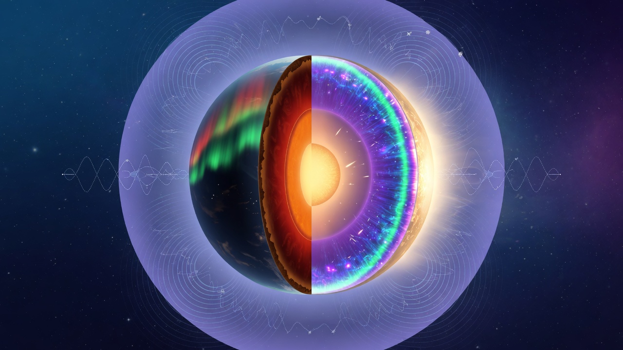
- Planetary weave shell stack
- Field Antenna JSON panels
- Phi versus RF disambiguation workshop
- Handoff discipline before Chapter 7 dispatch
Three meanings of RF in this stack
RF is three different weapons in the same word. Separate them or you will argue with a shader about ionospheric physics.
| Context | What RF means | Label |
|---|---|---|
planetary_weave.comp | Atmospheric visual shell layer | Visual |
| NEXUS Field Antenna | Local RF/audio/wired orchestration | Implemented |
Engine fieldPhi | Gate voltage / wave potential | Implemented |
Planetary weave — visual layer
Earth cross-section shader with concentric shells. RF layer sits in stack metaphor: core → crust → hydro → clouds → troposphere → ionosphere → RF shell → magnetosphere.
#define R_RF (R_EARTH + 1.05) // Layer L_RF — visual vocabulary
Visual vocabulary — teaches where signals live in stack metaphor. Does not compute FSPL inside AMOURANTHRTX shaders. Honesty on every rock.
What weave teaches
Pedagogy: operators need a picture of where defense and dispatch stories sit relative to atmosphere and ionosphere. Weave supplies picture, not instrument. When someone claims weave color proves propagation anomaly, return to Chapter 12.
fieldPhi — gate potential, not literal radio
Binding 8 Phi carries wave and gate potential — electrical metaphor coupled to Thermo and Flow. Implemented fabric evolution. claim that texels measure RF watts at antenna.
Chapter 3 coupling; Chapter 15 Maxwell tribute. Phi is RF word only in metaphor sense — label before you speak.
Field Antenna Orchestrator — NEXUS
Monitors RF + audio + wired + laser reference bands. Optical/laser entries 405–1550 nm. LIDAR flow ports in registry. GPS field anchors for triangulation metaphor. Outputs:
field-antenna-panel.jsonfield-rf-panel.jsonsignals-field-panel.json
Implemented in NEXUS. Local orchestration — correlate with packet field at panel :9477.
Registry and habits
Like port stories in Chapter 5, RF registry learns local device habits — context, not automatic verdict.
Free-space path loss — teaching reference
ITU-R/FCC context in NEXUS docs — not computed inside AMOURANTHRTX shaders. Teach path loss beside the label. Planetary weave does not replace FSPL math with colors.
Signals panel integration
Operator correlates signals-field JSON with packet field jsonl and AMOURANTHRTX THERMO — three scales from Chapter 2. No single dashboard metric collapse.
Queen and WebRTC — RF-adjacent perimeter
WebRTC is not disabled — gated through Connection Gatekeeper. RF words appear in peer stories; verdicts remain NEXUS. Chapter 21 Queen doctrine. MP4 mandatory in-tree; EME held.
Operator drill
./nexus.sh
curl -sk https://127.0.0.1:9477/signals-field-panel.json | head -c 1500
# Name which RF meaning each JSON block belongs to
Failure modes
| Mode | Symptom | Fix |
|---|---|---|
| Weave as instrument | Ionosphere claims from shader | Visual |
| Phi as MHz | Texel equals spectrum | Metaphor — binding 8 |
| FSPL in GPU | Expect FSPL in weave | NEXUS docs only |
| Antenna omniscience | Global RF vision | Local orchestration |
Chapter summary
RF is three meanings — weave visual, NEXUS antenna implemented, Phi potential implemented metaphor. FSPL is teaching reference. Planetary weave is vocabulary art. Chapter 7 offense dispatch next.
Study questions
- Fill three-row RF table from memory with labels.
- What does R_RF define — and what does it not compute?
- Name three Field Antenna JSON outputs.
- Why is FSPL not in AMOURANTHRTX shaders?
- How does Phi differ from planetary weave RF shell?
- Run signals panel drill — classify one JSON field.
- Cross-link Queen WebRTC gates — which chapter?
Chapter 7 — Offensive Dispatch →
Magnetosphere and ionosphere — visual stack only
Planetary weave stacks ionosphere then RF shell then magnetosphere as shader radii — pedagogy for where metaphorical signals sit. No claim AMOURANTHRTX models ionospheric scintillation for operations.
Audio bands in Field Antenna
NEXUS orchestrator includes audio alongside RF and wired — local device ecology, not Spotify analytics. Outputs land in signals panels for operator review.
Laser 405–1550 nm entries
Optical/laser registry bands are reference anchors — ITU/FCC teaching context in docs. Label before operational claims.
LIDAR flow ports
Registry includes LIDAR flow ports as habit context — correlate with packet field when local processes speak lidar-class ports.
GPS field anchors
GPS anchors support triangulation metaphor in signals layer — not replacement for survey-grade GNSS without labels. Pair with sovereign time Chapter 19 when sub-micron stories appear.
fieldPhi milli and gate stories
FIELD_PHI_MILLI = 618 and gate fidelity couple electrical metaphor to readable gates — implementation detail in engine headers. Not literal RF carrier frequency.
RetroRTX and planetary shaders
Specialty swipes may show planetary or retro visuals — still Visual unless stderr proves otherwise. Do not operationalize shader art.
Cross-link Chapter 7 offense
After RF separation, Chapter 7 dispatch writes fabric and die — offense continues stack. Defense read RF panels; offense writes Phi/Thermo/Flow. Same operator, different verbs.
ITU-R/FCC context in operator docs
NEXUS documentation may cite regulatory context for teaching FSPL and band plans — docs are not shaders. Teach beside label; grep implementation separately.
Extended treatment — planetary weave shader stack pedagogy
Core, crust, hydrosphere, clouds, troposphere, ionosphere, RF shell, magnetosphere — concentric radii in planetary_weave.comp. Each shell teaches where metaphorical signals live in Earth cross-section art. R_RF = R_EARTH + 1.05 defines RF layer radius — constant in shader literature, not ionosonde measurement.
Extended treatment — three RF meanings drill expanded
Drill daily until reflex: weave mention → Visual tag. Antenna JSON → Implemented NEXUS. Phi potential → Implemented fabric metaphor not literal MHz. FSPL equation → docs teaching only.
Extended treatment — Field Antenna Orchestrator bands
RF, audio, wired, laser 405–1550 nm, LIDAR ports, GPS anchors — local orchestration outputs to field-antenna-panel.json, field-rf-panel.json, signals-field-panel.json. Correlate with packet field; do not merge scores.
Extended treatment — fieldPhi gate potential
Binding 8 Phi — wave and gate potential, FIELD_PHI_MILLI 618 in engine vocabulary, GateFidelity coupling. Electrical words are metaphor; implementation is texel evolution. Chapter 15 Maxwell GPU coupling deepens.
Extended treatment — FSPL teaching beside implementation
FSPL ∝ 20 log10(d) + 20 log10(f) in ITU-R/FCC teaching context in NEXUS docs — not AMOURANTHRTX shader compute. Teach students beside label; quiz on label not on weave colors.
Extended treatment — Queen WebRTC and RF vocabulary
WebRTC peers produce packet sentences and may invoke RF words in UI — gatekeeper still owns verdict. MP4 in-tree; EME held. Chapter 21 completes browser perimeter; Chapter 6 prevents RF word collision errors before dispatch chapter.
RF chapter — examination preparation
Exam question: Define three RF meanings with labels. Exam question: Why is FSPL not in shaders? Exam question: Name three antenna JSON outputs. Exam question: What does R_RF define? Exam question: How does Queen handle WebRTC RF words? Pass by labeling every sentence.
Planetary weave is art for orientation — like classroom globe — not operational globe. Field Antenna is local instrument panel — like ham shack meters — not ionosonde network. Phi is fabric potential — like voltage metaphor in textbook — not voltmeter on PCIe.
Chapter 6 completes RF disambiguation before Chapter 7 dispatch — so when Phi moves, you do not claim ionosphere moved.
RF capstone — label every sentence drill
Sentence: Planetary weave shows ionosphere color. Label: Visual only. Sentence: Antenna panel lists band 915MHz entry. Label: Implemented NEXUS local. Sentence: Phi texel rose 0.3. Label: Implemented fabric metaphor. Sentence: FSPL at 2km 2.4GHz is X dB. Label: Teaching reference in docs. Sentence: Queen WebRTC peer connected. Label: Gatekeeper Implemented Chapter 21.
Five sentences, five labels, zero category errors — Chapter 6 exam passed.
Handoff: Chapter 7 dispatch writes Phi; you now know not to radio astronomer with shader screenshot.
Cross-links: 07-gpu-engine, 12-reality-theory, 15-maxwell-gpu, 21-field-browser-queen.
Planetary weave — layer walkthrough for instructors
Instructors teaching Chapter 6 should walk layers aloud: core, crust, hydro, clouds, troposphere, ionosphere, RF shell, magnetosphere. Each layer name is vocabulary only. Ask students: which layer is instrumented? Answer: none in AMOURANTHRTX shaders.
Field Antenna — correlating with packet field
When antenna JSON notes band activity and jsonl notes RX to matching port, human correlates — no auto-merge score. Same discipline as thermo plus packet correlation in Chapter 2.
Phi wave versus RF carrier — student confusion FAQ
Q: Is Phi 2.4 GHz? A: No — gate potential texel story. Q: Is weave color signal strength? A: No — visual. Q: Is antenna JSON dBm? A: Local orchestration reading — check implementation labels in NEXUS lib.
LIDAR ports registry — local habit context
LIDAR-related ports in registry provide habit context for robotics operators — not autonomous weapon narrative — local machine literacy.
GPS anchors and sovereign time
GPS field anchors meet sovereign time Chapter 19 when sub-micron stories appear — triple verify before trusting map dot pretty alone.
RF chapter hands-on — instructor checklist
Show weave screenshot — label Visual. Show antenna JSON — label Implemented. Show Phi heatmap — label fabric. Show FSPL in docs — label teaching. Quiz immediately.
Chapter 6 extended — RF disambiguation workshop (90 minutes)
Minutes 0-15: three meanings lecture. Minutes 15-30: planetary weave screenshot label Visual. Minutes 30-45: antenna panel JSON label Implemented. Minutes 45-60: Phi heatmap Classic label fabric metaphor. Minutes 60-75: FSPL worksheet from NEXUS docs label teaching. Minutes 75-90: exam five sentences from long_06c. Workshop completes before Chapter 7 dispatch.
Signals and packets — correlation without merge
signals-field-panel.json may show band activity same hour jsonl shows RX burst — write correlation paragraph, do not multiply scores into super-threat number. Human narrative discipline from Chapter 2 integration returns.
RF vocabulary for Queen operators
Queen UI may say WebRTC, ICE, codec, RF-adjacent words — gatekeeper still owns verdict. MP4 in-tree demux is packet parsing — Chapter 5 bytes perspective. Chapter 6 ensures RF word in UI does not bypass labels when you grep.
Handoff checklist to Chapter 7
Can you name three RF meanings? Can you quote FSPL is not in shaders? Can you label weave Visual? Yes — open Chapter 7 Offensive Dispatch. No — rerun workshop.
Introduction — three meanings of RF before you touch the spear
Operators arrive at Field Technology with one acronym and three incompatible intuitions. RF might mean the shader shell in planetary_weave.comp, the NEXUS Field Antenna orchestrator, or the wave potential on binding 8 — fieldPhi — that Maxwell language calls Φ, not megahertz. Chapter 6 separates them with honesty labels before Chapter 7 hands you vkCmdDispatch. Confusion here produces week-six embarrassment: ionosphere arguments from pretty colors, spectrum claims from jsonl panels, or radio astronomy from a Classic canvas screenshot.
Defense in Chapter 5 taught packet sentences. Entropy in Chapter 4 taught layer separation. This chapter teaches signal vocabulary — what is Visual, what is Implemented local orchestration, what is electrical metaphor on the fabric. The workshop protocol at chapter end is a lab you can run in an afternoon; the handoff to Chapter 7 states plainly: offense writes fields on the GPU; RF shaders do not replace dispatch literacy.
Learning objectives
- Label three RF contexts with correct status tags.
- Sketch planetary weave stack radii from core to magnetosphere.
- Read Field Antenna JSON panel outputs and correlate with packet field.
- Work FSPL teaching worksheet — ITU/FCC context, not shader compute.
- Disambiguate
fieldPhibinding 8 from literal radio propagation. - Execute workshop protocol and articulate handoff to Chapter 7.
Three meanings table — label before you speak
| Context | What “RF” means | Label | Product |
|---|---|---|---|
planetary_weave.comp | Atmospheric shell layer in Earth cross-section shader | Visual | AMOURANTHRTX |
| NEXUS Field Antenna | Local RF/audio/wired/laser orchestration + JSON panels | Implemented | NEXUS-Shield |
fieldPhi binding 8 | Wave / gate potential — electrical metaphor | Implemented + | AMOURANTHRTX |
planetary_weave.comp visual only.Queen WebRTC (Chapter 21) uses real network stacks behind gatekeeper — still not the same as weave shader art. WebRTC peers produce packet field sentences; planetary weave produces pedagogy pixels.
Planetary weave — stack radii from core to magnetosphere
planetary_weave.comp draws a concentric Earth cross-section — not a physics simulation of magnetohydrodynamics, a visual vocabulary for where signals “live” in the stack metaphor. Radii are shader constants; treat them as labeled shells in operator teaching, not satellite telemetry.
// Pedagogical shell stack (conceptual outer → inner)
core → crust → hydrosphere → clouds → troposphere
     → stratosphere → mesosphere → ionosphere
     → L_RF shell: #define R_RF (R_EARTH + 1.05)
     → magnetosphere → exosphere breath
The RF shell sits exterior to ionosphere in the narrative — a colored ring reminding you that propagation stories have a place in the stack without computing path loss in GLSL. R_EARTH anchors scale; R_RF offsets the teachable RF band as art. Swipe to weave canvas in AMOURANTHRTX when you want vocabulary; grep THERMO when you want dispatch truth.
Cross-link Chapter 15 Maxwell: binding 8 Phi participates in discrete Laplacian coupling on the fabric — neighborhood whispers, not ionospheric whistlers. Cross-link Chapter 9: FIELD_PHI_MILLI = 618 and GateFidelity sharpen gates — folklore mnemonic with a number, not a claim the universe prefers φ because the HUD said so.
Cross-link Chapter 12 honesty table: claiming the weave shader predicts HF skip zones is Visual accident marketed as instrument — refuse.
Field Antenna orchestrator — JSON panels that are real
NEXUS Field Antenna is Implemented local orchestration across RF, audio, wired, and optical reference bands. It watches flows and anchors meaningful to your machine — not global spectrum survey.
- Optical / laser reference entries: 405–1550 nm teaching bands
- LIDAR flow ports registered beside socket habits
- GPS field anchors for triangulation metaphor — not replacement for survey grade receivers
- Outputs:
field-antenna-panel.json,field-rf-panel.json,signals-field-panel.json
Panel :9477 Signals tab (Chapter 5) surfaces these artifacts. Correlate JSON rows with field jsonl sentences — same peer, same sealed time column, different views. No merged super-score. Field Antenna does not replace gatekeeper verdicts; packet field does not replace FSPL homework.
| JSON artifact | Typical content | Correlate with |
|---|---|---|
field-antenna-panel.json | Antenna path registry, band tags | Signals tab, local hardware |
field-rf-panel.json | RF flow summaries, habit notes | Packet field port axis |
signals-field-panel.json | Cross-domain signal map | Chapter 5 defense rhythm |
FSPL teaching worksheet — path loss on paper, not in shaders
Free-space path loss (FSPL) belongs in operator notebooks and NEXUS teaching docs — not inside AMOURANTHRTX fabric shaders. ITU-R and FCC contexts use:
Distance d grows loss with twenty log ten; frequency f does the same. Double distance costs ~6 dB; double frequency costs ~6 dB. The worksheet builds intuition before you touch hardware.
# Given: f = 2.4 GHz Wi-Fi, d = 10 m (free space teaching model)
# FSPL ≈ 20*log10(10) + 20*log10(2.4e9)  [use consistent units in your notebook]
# Compare: d = 100 m — how many dB added vs 10 m?
# Label answer: teaching estimate — not measured in planetary_weave.comp
Worksheet 6.B: repeat for 915 MHz ISM at 1 km. Worksheet 6.C: explain why attic copper foil does not change shader R_RF constant — visual shell unchanged by real-world sheet metal.
Chapter 6 honesty: FSPL exercises train judgment for Field Antenna context. They do not authorize claims that Classic canvas color maps predict link margin.
Phi versus RF — disambiguation clinic
fieldPhi on binding 8 is the analog fabric’s wave and gate potential channel. Shaders read and write Φ per texel; host packs WaveSpeed, GateFidelity, PropalacticScale into FCC floats. This is Maxwell neighborhood on a grid — Chapter 15 — not literal RF carrier tracking.
| Question | Phi / binding 8 | RF / Field Antenna | Weave shader |
|---|---|---|---|
| Measured in MHz? | No — arbitrary field units | Band labels for orchestration | No — art scale |
| Where grep? | THERMO + fabric + FCC slots | NEXUS JSON + jsonl | Canvas swipe only |
| Honest label | Implemented metaphor | Implemented local | Visual |
| Couples to Thermo? | Yes — FieldCoupling | Indirect via machine activity | No — decor |
Clinic sentence: “Phi gradient steepened, so RF must be jammed” is category error. “Field Antenna noted 2.4 GHz habit breakage on RX, gatekeeper SUSPICIOUS” is legible defense. “Ionosphere glow red on weave” is art critique, not propagation measurement.
Workshop protocol — afternoon lab
- Label pass (15 min): List three RF meanings from memory; tag each Visual, Implemented, or .
- Weave swipe (20 min): Open AMOURANTHRTX planetary weave canvas; sketch shell stack on paper with
R_RFnoted; refuse FSPL claims from colors. - FSPL worksheet (25 min): Complete 6.A–6.C on paper; photograph page for operator journal — not for vendor slide deck.
- NEXUS panels (30 min):
./nexus.sh; open :9477 Signals; read three JSON artifacts; tail matchingfield jsonlrows. - Phi grep (20 min):
./linux.sh run;set AnalogFields.GateFidelity 0.9; grep THERMO + FCC; confirm fabric offense path alive — handoff prep. - Disambiguation drill (10 min): Write three sentences — one correct per layer; one deliberate category error; fix the error aloud.
Ionosphere and magnetosphere — teachable shells, not predictions
In the weave narrative, ionosphere and magnetosphere rings sit outside troposphere weather and inside exosphere breath. They exist so instructors can point at a screen and say: “HF stories live in sky vocabulary; your loopback panel lives in operator vocabulary.” The shader does not compute critical frequency, foF2, or K-index. It paints teachable regions.
When a student asks whether red ionosphere glow means solar storm, answer with labels: Visual pedagogy. Then open :9477 and show jsonl habits — defense receipts. Then run ./linux.sh run and grep THERMO — offense receipts. Three layers, three answers, one disciplined operator.
Chapter 10 spiderweb mirror uses fabric averages, not ionosphere colors. Chapter 6 refuses the shortcut that makes pretty globes feel like NOAA products.
Queen, WebRTC, and RF words in UI
Queen holds WebRTC gates (Chapter 21). RF vocabulary in UI still passes Connection Gatekeeper — honorability axis asks whether navigation context matches socket reality. Field Antenna may tag RF bands; packet field records peers; thermo proxy records dispatch cost on Queen build — parallel witnesses, not one score.
MP4 mandatory in-tree means media paths are not outsourced to CDN conscience — local archive discipline matches jsonl ethos. EME held, not omitted, because sovereign browser doctrine refuses hole-poking.
Failure catalog — RF edition
| Failure mode | Symptom | Fix |
|---|---|---|
| Weave as instrument | HF propagation forecast from shader | Visual rock — Ch. 12 |
| Phi as MHz | “Tune binding 8 to 2.4G” | FCC floats are field knobs, not carrier |
| FSPL in GLSL fantasy | Expect path loss in fabric | Paper worksheet only |
| JSON super-score | Merge antenna JSON + gatekeeper | Correlate; separate verdicts |
| GPS metaphor as survey | Sub-centimeter claims from anchors | Label triangulation metaphor |
| Disable WebRTC | Queen security hole-poke | Ch. 21 hold gates |
| Cloud RF omniscience | NEXUS sees planet spectrum | Local-first — Ch. 5 |
| Skip workshop | Jump to Ch. 7 without labels | Run protocol once |
Audio, wired, and optical bands — one orchestrator, many witnesses
Field Antenna does not stop at textbook RF. Local orchestration includes audio device paths, wired interface habits, and optical reference bands from 405 nm through 1550 nm — teaching anchors for laser and LIDAR vocabulary on your machine. Each band entry is a labeled witness in JSON, not a claim NEXUS measured photons in your fiber run.
LIDAR flow ports in the registry sit beside TCP habits: a UDP burst on a registered port may correlate with a signals-field row without merging into gatekeeper verdict math. GPS field anchors supply triangulation metaphor for panel maps — useful pedagogy when teaching children the difference between “where the UI drew a dot” and “where survey equipment proved a coordinate.”
When Signals tab shows optical entries alongside RF summaries, practice the Chapter 5 rule: correlate timestamps with field jsonl, compare process paths, refuse single-score dashboards. Field Technology trains parallel reading — thermo stderr, packet sentences, antenna JSON — the operator integrates.
Propagation vocabulary without instrument fantasy
Operators need words for sky and wire even when shaders are art. Teach vocabulary honestly:
- Ground wave — metaphor for local wired habits and loopback flows; grep jsonl, not weave colors.
- Sky wave — ionosphere story in planetary weave shell; Visual only.
- Free space — FSPL worksheet domain; paper and calculator, not
fieldPhitexels. - Multipath — real Wi-Fi frustration; Field Antenna may note band congestion patterns locally without predicting shader palette.
Chapter 14 Shannon surprise on encrypted payloads sometimes correlates with “noise floor” stories — still not weave red pixels. Keep layers separated as Chapter 4 demands.
Handoff to Chapter 7 — offense takes the spear
You labeled three RF meanings. You correlated Field Antenna JSON with packet field sentences without merging scores. You worked FSPL on paper while refusing shader compute fantasy. You disambiguated Φ on binding 8 from literal radio.
Chapter 7 is next: thin host, fat GPU, Pipeline::dispatch_canvas() → vkCmdDispatch. Default canvas is x86.comp with Field Die — offense writes guest RAM, fabrics, thermo receipts every tick. Planetary weave taught vocabulary; dispatch teaches sovereignty.
Defense (Ch.5) read jsonl → RF (Ch.6) labeled meanings → Offense (Ch.7) vkCmdDispatch
Carry forward: stderr before screenshots, rocks before poetry, grep before argument. ThermoAccountant from Chapter 4 still populates binding 2 on every dispatch — RF clarity does not pause thermo obligation.
Continue: Chapter 7 — GPU Field Engine. Prior: Chapter 5 — Packet Field. Rocks: Chapter 12. Maxwell creditor: Maxwell.
Chapter summary
RF in this stack names three different stories: planetary weave visual shell at R_RF, NEXUS Field Antenna local orchestration with JSON panels, and fieldPhi wave potential on binding 8 as implemented electrical metaphor. FSPL works on teaching worksheets — not in fabric shaders. Workshop protocol trains label discipline. Chapter 7 inherits operators who will not confuse ionosphere art with dispatch truth.
Deep dive — ITU-R and FCC as teaching context, not shader constants
NEXUS documentation cites ITU-R and FCC framing for path loss, band plans, and operator vocabulary — teaching context beside local jsonl scope. The citations exist so instructors can assign worksheets without pretending AMOURANTHRTX shaders became spectrum regulators.
When students ask “is this legal on 5 GHz,” answer: consult counsel and national regulators; Field Primer teaches technical honesty and local perimeter, not legal advice. When students ask “does weave red mean illegal transmit,” answer: Visual only — check Field Antenna JSON and jsonl for real local sense layers.
Deep dive — spectrum analyzer honesty for advanced labs
External USB analyzers may join advanced operator labs — hardware outside the stack. If you capture a trace, label it External instrument distinct from planetary weave screenshots and distinct from fieldPhi heatmaps. Three images, three labels, one collage grade in Exercise 6.C.
Never paste analyzer traces into threat dashboards as auto-verdicts. Correlation paragraph only: “Analyzer peak at time T; jsonl RX burst at T±2s; weave screenshot unrelated.”
Chapter 11 observability extends grep rhythm to RF labs — archive traces with session IDs like thermo journals.
Deep dive — teaching children and newcomers RF discipline
Children learn labels faster than they learn Vulkan. Start with three-card drill: Visual, Implemented, Metaphor. Planetary weave card says Visual. Field Antenna card says Implemented local JSON. Phi card says Implemented fabric metaphor. FSPL worksheet card says Paper math.
Adults skip cards and skip labels — then argue across layers at dinner. Chapter 6 exists to front-load the argument you would otherwise have at midnight on Discord.
Deep dive — planetary weave shader stack as literature
Open planetary_weave.comp as literature, not instrumentation. Radii constants name shells — core, crust, hydrosphere, clouds, troposphere, ionosphere, R_RF, magnetosphere — each a pedagogical ring. The RF shell is one radius in a stack metaphor, not a measurement of watts exiting your Wi-Fi antenna.
Color choices encode mood: warm ionosphere, cool magnetosphere, cloudy troposphere. Mood is not METAR. When instructors assign “read the stack,” students should sketch rings on paper and label each Visual before discussing NEXUS Field Antenna JSON.
Swiping to weave in AMOURANTHRTX does not pause Field Die default product truth — weave is alternate curriculum on shared Vulkan spine per Chapter 7. Thermo still accrues underneath; THERMO still greps.
Deep dive — Field Antenna operator tour (30 minutes)
- Start NEXUS; open Signals tab at :9477.
- Load
field-antenna-panel.json— note schema version in file header if present. - Compare
field-rf-panel.jsonversussignals-field-panel.json— different slices, same honesty rule: correlate, no super-score. - Record one audio device entry, one wired entry, one optical reference band entry — three labels, three sentences.
- Open Classic Phi heatmap in AMOURANTHRTX — fourth image in collage; label fabric metaphor.
- Complete FSPL worksheet for hypothetical 2.4 GHz link at 10 m — paper only.
- Write handoff sentence: “Phi is binding 8; weave is Visual; antenna is local JSON.”
Tour completes Chapter 6 workshop; archive notes beside jsonl, not instead of jsonl.
Deep dive — magnetosphere and exosphere as narrative bookends
Outside RF shell, magnetosphere and exosphere rings teach that signals live inside stories about space — not that shaders predict solar wind pressure. Narrative bookends bracket the RF chapter: inner shells ground newcomers in geography metaphor; outer shells remind that hype expands outward unless labels contract it.
Chapter 17 God at holographic boundary and Chapter 6 planetary weave both use cosmic vocabulary — different jobs. Chapter 17 sacred long-form; Chapter 6 category discipline. Do not merge them into one cosmology slide without rocks.
Deep dive — RF chapter closing ritual before dispatch
Before opening Chapter 7, run this sixty-second ritual:
- Say aloud: “Weave is Visual.”
- Say aloud: “Antenna JSON is local Implemented.”
- Say aloud: “Phi is fabric metaphor on binding 8.”
- Say aloud: “FSPL is paper, not GLSL.”
- Grep one THERMO line — offense prep reminder.
- Archive one jsonl row if NEXUS running — defense prep reminder.
Ritual sounds silly until the third week when someone cites ionosphere color as threat intel. Chapter 6 buys you immunity to that meeting.
Study questions
- Tag three RF contexts with correct honesty labels.
- Where does
R_RFsit in the shell stack narrative? - Name three Field Antenna JSON outputs and panel tab.
- Write FSPL proportionality; why not in
x86.comp? - Give one Phi vs RF category error and correction.
- Complete workshop protocol step 5; what grep proves offense prep?
- Why no merged super-score between JSON and gatekeeper?
- How does Queen treat WebRTC versus weave shader?
- Which failure mode matches “forecast from weave colors”?
- State handoff sentence from Chapter 6 to Chapter 7.
Planetary weave comp stack order
Core to magnetosphere ordering teaches concentric thinking — RF shell one radius among many, not the whole story.
Cloud layer versus troposphere
Visual weather shells are not weather API — no METAR in shader.
Hydrosphere metaphor
Water shell pedagogy for signal environment metaphor — still visual.
Crust and core — geophysical art
Geophysical art sets mood for RF chapter — separates mood from measurement.
Antenna panel JSON schema stability
Panel JSON versions may evolve — grep schema version in file when correlating old archives.
RF panel versus signals panel
field-rf-panel versus signals-field-panel serve different slices — read filenames literally.
Phi wave speed versus RF propagation
WaveSpeed knob is fabric stability parameter — not speed of light in ionosphere.
Maxwell Chapter 15 handoff
After RF separation, Maxwell GPU chapter deepens Phi/Thermo coupling math story — read order 6 then 15.
NEXUS docs FSPL examples
Worked FSPL examples live in docs for teaching — copy to lab notebook, not to shader constants.
RF vocabulary disambiguation drill
Drill: speaker says RF spike. Ask which RF — weave visual? antenna JSON? Phi potential? Politeness with insistence on label.
Planetary weave shader constants
R_RF and stack radii are #define pedagogy — read shader as literature with labels, not instrumentation datasheet.
Signals triangulation metaphor limits
GPS anchors in signals field support metaphorical triangulation stories — not survey grade without external proof.
Audio RF wired laser — one orchestrator
Field Antenna Orchestrator unifies spectrum of local sense layers — unify in panel, separate in labels.
Phi-Thermo-RF word collision
Phi uses electrical words; weave uses RF words; antenna uses RF words — glossary Chapter 22 will disambiguate; Chapter 6 starts fight early.
Exercise 6.C — label collage
Screenshot weave, antenna panel, Classic Phi heatmap — paste three honesty labels under each image. Visual collage discipline.
Handoff to GPU engine chapter
Chapter 7 dispatch writes Phi that Chapter 6 refuses to confuse with ionosphere. Read next with RF separation loaded.
Evidence anchor — grep and sources
Major claims in this chapter anchored for reproducibility. Implemented = grep today; = intuition; Philosophy = discipline.
| Claim | Statement | Label | Evidence |
|---|---|---|---|
| Planetary weave | RF shell shader art | Visual | planetary_weave.comp |
| Field Antenna | JSON RF panels | Implemented | Field Antenna module |
| Phi binding 8 | Fabric potential | Not spectrum analyzer | |
| FSPL | Free-space path loss | Paper equation — not in shader SI |
FSPL ∝ 20·log₁₀(d) + 20·log₁₀(f) | R_RF shell layer (visual)
grep -r 'planetary_weave' Navigator/shaders/
Source paths
Navigator/shaders/planetary_weave.compNEXUS-Shield/field_antenna.json
Chapter summary — before you turn the page
Three RF meanings labeled: weave Visual, antenna Implemented, Phi fabric metaphor. FSPL stays on paper. Workshop complete — open Chapter 7 with dispatch literacy loaded.